
As you already know by now, Excel is among, if not the most powerful piece of software that can assist individuals and businesses in making the job of accountants easier by significantly streamlining the accounting and financial control processes that they undertake.
For one, with its various functions and formulas, Excel allows accountants to efficiently track financial data, thus effectively saving precious company time and improving accounting accuracy. In addition, the software is famous because it can assist in managing financial records by making it easier for accountants to analyze and understand all types of financial information. Besides, Excel can automate tasks such as tracking income, expenses, and other financial data, making it a powerful tool for financial analysis and decision-making.

From Unsplash
For an accountant, mastering Excel and knowing how to use the most famous accounting formulas can significantly enhance your abilities in managing and analyzing financial information. This Excel training guide will provide you with the fundamental knowledge and resources that you require to take your Excel game to the next level, regardless of whether you are a proprietor of a small business, a financial analyst, or just a visitor who is interested in gaining a better understanding of their finances over a certain period.
The following formulas can help automate the tracking of income, expenses, and other types of financial data and resources. They can also make it simpler to analyze and comprehend your financial information, which is essential for every accountant or business owner to make informed financial decisions. So, let’s get started!
The asset depreciation formula
With the help of Excel, you can quickly start calculating asset depreciation and find the right amount of value that an asset will eventually lose over time. To do that, Excel provides five different ways in which you can calculate asset depreciation:
- Straight-line depreciation (cost, salvage, life). The SLN calculation can reveal the asset’s value lowering by a fixed period over its life.
- Decline balance depreciation (cost, salvage, life, period, month). This formula can be utilized to reduce the asset’s value by a fixed percent, where the monthly value is optional.
- Variable decline balance depreciation (cost, salvage, life, start period, end period, factor, no switch). The last two values here (factor and no switch) are optional. This formula can help you provide depreciation over a user-specified time.
- Double decline balance depreciation (cost, salvage, life, period, factor). This formula can help you double the rate of straight-line depreciation, where the factor value is optional.
- The sum of years’ depreciation (cost, salvage, life, per). The SYD formula can show you a given item’s declining value over a number of years.
To give a real-life example, let’s say that your boss wants to purchase a brand new car for $20,000, and they want to know how much the car will depreciate in the first seven years of its life. To calculate that, you need to use the declining balance depreciation formula.
The salvage value of the car is $1,400, that being the value after the vehicle’s depreciation. The estimated life expectancy of the car your boss wants to get is 20 years. To calculate the depreciation value of the car, you’ll use the declining balance depreciation formula =DB (20,000 – 1,400) x 7% and find that it equals $1302,00.

From Pexels
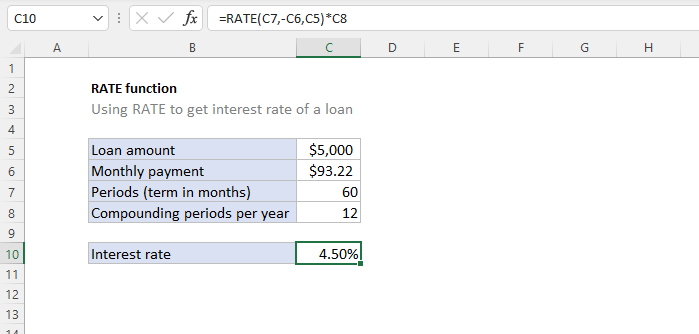
Calculating annual interest rate in Excel with the RATE function
Next in line, you can utilize the RATE function in Excel to calculate any given annual interest rate for a business loan. For example, the formula here would be:
RATE (number of payment periods; the amount paid toward the loan each year; the present loan value; the loan balance after the final installment; the optional argument for when the loan payment is due; and the user’s guess for the rate—a value that defaults to 10%).
So, if your boss wants to understand what their annual interest rate is on a $5,000 loan that they pay off with $93.33 per month for five years (sixty months), you can use the formula =RATE (60, -750, 5,000)*12 and determine that the annual loan interest rate is 4.50%.
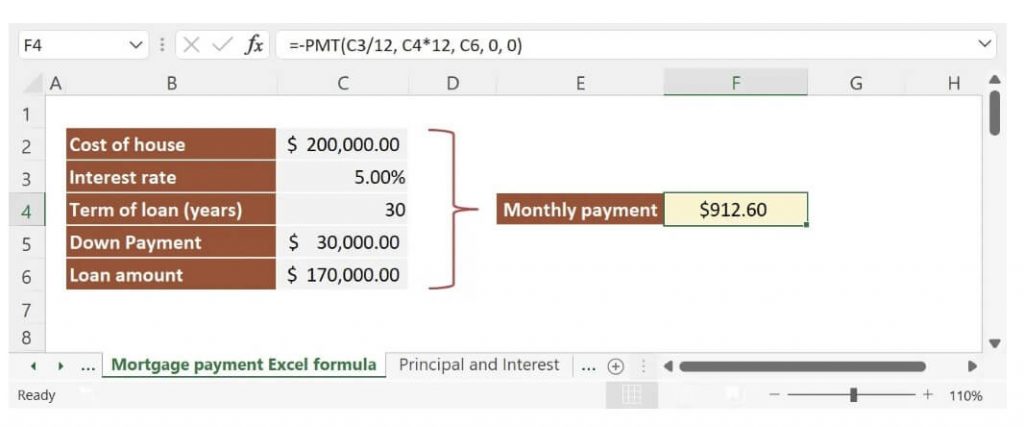
Business mortgage payments formulas in Excel
Furthermore, you can also use the PMT function and create a customized formula to identify the cost of a potential mortgage payment. For example, the Excel formula here would be:
PMT (the interest rate for the loan; the number of loan payments due; the loan principal amount; the cash balance after the last installment, which is optional, and if you don’t include such value, it defaults to zero; and when the loan payment is due.)
So, if your boss wants to invest in a new business office with a 30-year, $170,000 business mortgage loan to be repaid monthly, with the loan interest rate being 7%, using the PMT formula, you can easily calculate the monthly loan payment: =PMT(5% (the loan interest rate) /12 (twelve monthly payments), 30 (term of the loan in years)*12, 170,000 (loan amount) to find that your boss would owe a monthly fee of $912.60.
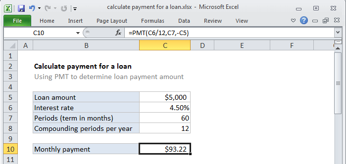
Calculating fixed loan payment data
Thanks to the IPMT function in Excel, you can also easily calculate the portion of interest on a loan payment on behalf of your company or for your client. Here, the IMPT formula would be:
IMPT (the loan interest rate; the interest period; the number of loan payments due; the loan principal amount; the cash balance after the last installment, an optional value; and the time when the loan payment is due).
So, if a client of yours wants you to find the portion of interest on a five-year, $5,000 loan payment with 4.5% interest that their company pays monthly, you can use the formula =IMPT ((4.5% (the interest rate) / 12 (compounding periods per year), 60 (total payment periods), -5,000)) to find that the monthly payment will be $93.22.
Formulas for calculating compound interest
As you probably already know, compound interest is the inclusion of interest in a loan’s principal sum. Frequently, compound interest is described as interest earned on interest. So, if you want to find the actual future value of an investment, you can use a compound interest formula in Excel.
The formula here would be: p*(1+r)^n, where P stands for the principal loan amount, R stands for the loan interest rate , and N stands for the investment period of the loan.
To put this formula into perspective, if a client wants to take a personal loan of $1,000 to be paid at 8% over four years, you can use the formula to calculate their compound interest. For example, using the formula =1000*(1+8%)^4, you can figure out that the compound interest on the loan would be $1,166.40.

From Unsplash
Final thoughts
In conclusion, Excel is a powerful tool that functions by helping businesses and individuals streamline their financial management processes. The resources and formulas covered in this guide can help automate the process of tracking various finance-related data and make it easier to analyze and understand this process.
By mastering these formulas, you can save time, reduce errors and make better decisions. Remember that these formulas are just the beginning; Excel has many other functions and features that can help you analyze your information more deeply, so keep learning and exploring.